In the investment world, it’s common to discuss average rates of return. It’s not sufficient, however, to simply add up historical returns and divide by how many there are.
The proper way to calculate average investment returns is with a geometric mean that takes into account the compounding effects of a series of volatile returns over time. But crucially, the assumption of volatility always produces some level of drag on projected returns. This can make it difficult — though no less crucial — for advisors to be cognizant of whether they are unwittingly entering lower-than-intended return assumptions in their retirement projections.
The most common version of an average, taught to children in their early school days, is the arithmetic average or arithmetic mean — calculated by adding up all the individual items and dividing by how many there are.
This is effective in situations where the items being measured are independent of one another. The height of one student does not have any impact on the heights of the other students, and the exam score of one test taker doesn’t have any relationship to the others.
By contrast, in the world of investment returns, the results of one year are related to the results of the next, because both are being compounded on a dollar amount that grows in Year No. 1 before being reinvested or continuing to be held for investment in Year No. 2. As a result, a simple arithmetic return fails to capture the compounding effects that occur from a sequence of investment returns.
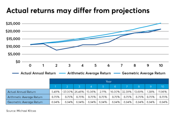
Example 1. From 2007 to 2016, the S&P 500 has posted
And yet, an actual $10,000 investment in the S&P 500 over this time would have grown to only $19,568.08. The fact that the first year’s return was 5.49% meant that by Year No. 2, there wasn’t $10,000 invested to experience the -37% decline; rather, there was $10,549. And by the third year, there wasn’t $10,000 invested to experience the 26.46% recovery, as the portfolio would have been down to $6,645.87. And by the fourth year, the 15.06% return would have been experienced on only the $8,404.37 balance from the end of the prior year. And, so forth.

In other words, each year’s return carries over to impact the balance being invested into the subsequent year, meaning that it’s not enough to merely add up the returns of each year and divide by how many there are to determine the average rate of portfolio growth. Instead, the actual average return is somewhat lower to account for the fact that there were both higher and lower returns that compounded along the way. This is known as the geometric mean, or the geometric average return.
The geometric average represents the average annual growth rate that would have generated an equivalent amount of final wealth with a straight-line series of returns, even though the returns didn’t actually occur in a straight line.
Also known sometimes as the annualized return or the compound average growth rate, the geometric average return may not match the actual return in any particular year, but by definition, it will compound into equivalent cumulative wealth at the end of the time period. In the earlier example, the geometric return or CAGR would have been 6.94%.

As shown in the example above, the geometric return was lower than the arithmetic return by about 1.81%, due to the fact that the compounded volatile returns with the early bear market never quite added up to what the straight line return would have been. However, this difference isn’t unique to just this particular series of volatile returns with a bear market.
Indeed, any level of ongoing volatility will cause the geometric average to lag its arithmetic mean counterpart.
Example 2. From 2007 to 2016, the annual returns of the
Notably, the geometric average return in this example was only very slightly lower than its arithmetic mean counterpart. Nonetheless, even with a less volatile sequence that had only good compounding returns up front, the geometric mean was still lower.
The inevitable gap between the arithmetic mean and the geometric average return is often called volatility drag. Mathematically, the more volatile the returns are, the more of a gap there will be. That said, the exact amount of volatility drag will vary by the exact sequence of returns and amplitude of the volatility. It can be approximated, however, by subtracting half of the variance from the arithmetic mean, where variance is the standard deviation squared, or conversely standard deviation is the square root of variance.
Example 3. The standard deviation of the S&P 500 return series was 18.86%, which equates to a variance of 3.56%. On the other hand, the Barclays Aggregate Bond returns had a standard deviation of 3.12%, or a variance of 0.10%. Accordingly, this implies that with an arithmetic average return of 8.75% on the S&P 500, the geometric return would be 8.75% - 3.56% / 2 = 6.97%. That is quite close to the actual geometric mean of 6.94%. Similarly, the Barclays Aggregate Bond had an arithmetic return of 4.39%, which would be reduced by 0.10% / 2 to an estimated geometric mean of 4.34%. That in turn is very close to the actual geometric mean of 4.35%.
Practically, the estimation of the geometric mean from its arithmetic counterpart and the standard deviation and variance may not perfectly align. A limited set of data points may not exactly conform to the underlying normal distribution on which this formulaic assumption is based. Nonetheless, as shown in the examples above, it is typically very close — in this case, within three basis points for the geometric return of a 10-year series of stock returns, and within one basis point for the geometric average of the 10-year bond returns.
The impact of volatility on compounded arithmetic return is often called a volatility drag, or a variance drain. While this force may reduce returns to arrive at a lower geometric average return, the reality is simply that the arithmetic mean is an inaccurate way to describe long-term compounded returns.
Fortunately, in practice virtually all returns discussed in the context of investments are already based on the geometric mean — whether it’s a CAGR or a discussion of the annualized returns. And both time-weighted and dollar-weighted returns are inherently measures of the CAGR in a portfolio.
However, the fact that returns — as typically discussed — are based on geometric returns indicates that advisors must still be cautious in how they translate rates of return into appropriate assumptions to use in forward-looking retirement projections.
When doing a traditional, straight-line retirement projection that estimates future wealth based on some average annual compound growth rate — along with ongoing contributions or withdrawals — the geometric return is the appropriate return to use because it’s the one that would produce the correct compounded dollars at the end of the time period.
However, when it comes to Monte Carlo assumptions, the proper return assumption is the arithmetic mean, not the geometric average return. Indeed, the whole point of Monte Carlo analysis is not just to estimate the straight line return to reach final wealth, but to actually project the results of a series of randomly drawn, and therefore volatile, returns based on the probability that they occur.
In other words, the gross arithmetic average returns that are plugged into a Monte Carlo analysis will automatically be reduced to the equivalent geometric returns in the process of projecting annual volatility. This means that if the geometric average return is the starting assumption along with a standard deviation volatility assumption, and then a random series of Monte Carlo returns are drawn based on that underlying volatility, the end result will be retirement projections whose geometric returns are lower than intended.
Example 4. Jeremy is running a 30-year retirement projection for a 65-year-old client, where stocks are assumed to have an average annual growth rate of 10% and bonds are assumed to grow at 5% — consistent with their long-term
In order to achieve a Monte Carlo analysis where the final geometric return is consistent with the desired long-term averages, Jeremy should have gone back to the original data to calculate the higher arithmetic average on which the returns were based, or alternatively just increased the return assumptions by half of the variance to estimate the original arithmetic return. This would have produced an assumed arithmetic return of 11.45% for stocks and 5.25% for bonds — such that, after including the impact of volatility drag, the final returns would have ended out at approximately 10% for stocks and 5% for bonds.
And notably, the cumulative impact of this difference is substantial. If the client had a 50/50 portfolio, the client’s long-term compounded returns would be only 6.65% — or slightly higher with a
In turn, had Jeremy planned to take a 5% initial withdrawal rate, a proper Monte Carlo analysis based on historical arithmetic means would have had an 87% probability of success — and the proper long-term compounded return — but one that used the geometric return up front, as though it was an arithmetic mean, even when it isn’t. It would have only an 76% probability of success, with a long-term return substantially below what the geometric return was supposed to be.

As the graphic above shows, when geometric returns are used as a Monte Carlo input, the final results produce lower returns than intended, resulting in a higher probability of failure, as the projection effectively double-counts the impact of volatility drag. This is because geometric returns already include volatility drag, and using geometric returns in a Monte Carlo projection just adds a second layer of drag when the software re-projects the future impact of volatility. By contrast, when arithmetic returns are used as the assumption up front, the final results are consistent with the geometric returns expected in the end.
Of course, in today’s environment of high market valuations and low yields, many advisors may wish to use below-historical-average returns
On the other hand, some Monte Carlo software tools already increase geometric returns to their arithmetic counterpart behind the scenes — using a version of the approximation noted above — recognizing that arithmetic returns are the proper assumptions, but that most advisors by default discuss and use geometric returns.
This means that the software may actually be projecting correctly, having adjusted for the advisor’s default geometric return assumption. But at a minimum, it’s crucial to clarify for any particular Monte Carlo retirement projection what return assumptions are actually being used, and whether it is the proper arithmetic return being iterated on in the random Monte Carlo return draws.
The bottom line though is simply to recognize the important difference between arithmetic and geometric return assumptions, both in the general case of describing and explaining returns — and the role of volatility drag — and especially given the unique effect that variance drain can have on Monte Carlo projections in particular.
And this of course makes it especially important to input the right version of a return assumption up front when projecting a retirement plan.
So what do you think? What are the return assumptions that you use in a retirement plan? Are they based on arithmetic or geometric average returns? Are you going to adjust your return assumptions going forward? Please share your thoughts in the comments below.


